Many mathematicians, from Archimedes to Leibniz to Euler and beyond, made use of infinitesimals in their arguments. These were later replaced rigorously with limits, but many people still find it useful to think and derive with infinitesimals.
Unfortunately, in most informal setups the existence of infinitesimals is technically contradictory, so it can be difficult to grasp the means by which one fruitfully manipulates them. It would be useful to have an axiomatic framework with the following properties:
1. It is consistent.
2. The system acts as a good “intuition pump” for the real world. In particular, this entails that if you prove something in the system, then while it won’t necessarily be true in the real world, there should be a high probability that it’s morally true in the real world, i.e., with some extra assumptions it becomes true. It should also ideally entail that many of the proofs of Archimedes, et al., involving infinitesimals can be formulated as is (or close to “as is”).
“Smooth infinitesimal analysis” is one attempt to satisfy these conditions.
(This is a blogified version of the first part of an article I wrote here.)
Axioms and Logic
Consider the following axioms:
Axiom 1. 


Furthermore, we have that 
Axiom 2. There is a transitive irreflexive relation 


It also satisfies 
Axiom 3. For all 


Axiom 4 [Kock-Lawvere Axiom]. Let 


After reading the Kock-Lawvere Axiom you are probably quite puzzled. In the first place, we can easily prove that 


For an alternate proof that 


Now, if 
However, we have the following surprising fact.
Fact. There is a form of set theory (called a local set theory, or topos logic) which has its underlying logic restricted (to a logic called intuitionistic logic) under which Axioms 1 through 4 (and also the axioms to be presented later in this paper) taken together are consistent
Definition. Smooth Infinitesimal Analysis (SIA) is the system whose axioms are those sentences marked as Axioms in this paper and whose logic is that alluded to in the above fact.
References for this theorem are [Moerdijk-Reyes] and [Kock]. References for topos logic specifically are [Bell1] and [MacLane-Moerdijk].
Essentially, intuitionistic logic disallows proof by contradiction (which was used in both proofs that 

I won’t formally define intuitionistic logic or topos logic here as it would take too much space and there’s no real way to understand it except by seeing examples anyway. If you avoid proofs by contradiction and proofs using the law of the excluded middle (which usually come up in ways like: “Let 


But before we go further we might ask, “what does this logic have to do with the real world anyway?” Possibly nothing, but recall that our goals above do not require that we work with “real” objects; just that we have a consistent system which will act as a good “intuition pump” about the real world. We are guaranteed that the system is consistent by a theorem; for the second condition each person will have to judge for themselves.
To conclude this section, it should now be clear why I didn’t want to call
Even though we have 

For the rest of this blog entry I will generally work within SIA (except, obviously, when I announce new axioms or make remarks about SIA).
Single-Variable Calculus
An Important Lemma
This lemma is easy to prove, but because it is used over and over again, I’ll isolate it here:
Lemma [Microcancellation] Let 


Proof.
Let 

Basic Rules
Let 


We thus have the following fundamental fact:
Proposition [Fundamental Fact about Derivatives]
For all 
and furthermore,
Proposition Let 

1.

2.

3.
4. If for all 

5. 
Proof
I’ll prove 3 and 5 and leave the rest as exercises.
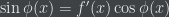
To prove 3: Let 

which, multiplying out and using 

On the other hand, we know that 

Since 
To prove 5: Let

Now, 


As before, this gives us that 

In order to do integration, let’s add the following axiom:
Axiom 5 For all 


We can now derive the rules of integration in the usual way by inverting the rules of differentiation.
Deriving formulas for Arclength, etc.
I’d now like to derive the formula for the arclength of the graph of a function 

For this problem, and other problems which use geometric reasoning, it’s important to note that the Kock-Lawvere axiom can be stated in the following form:
Proposition [Microstraightness] If 


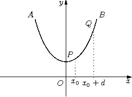
Let 

Let 
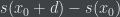


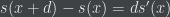
Because of microstraightness, we know that the part of the graph of 


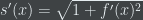
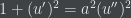
To determine the length of 

The hypotenuse of a right triangle with legs of length 1 and 


So, we know that 


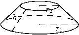
Several other formulas can be derived using precisely the same technique. For example, suppose we want to know the surface area of revolution of 


Then, let 


which, multiplying out, becomes 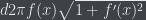


In a precisely analogous way, one may derive the formula for the volume of the solid of revolution of 


Above we assumed that we knew the surface area of a frustum of a cone. Finally, as an exercise, eliminate this assumption by deriving the formula for the surface area of a cone (from which the formula for the surface area of a frustum follows by an argument with similar triangles) as follows:
Fix a cone 


Let 

Using a method similar to that above, determine that 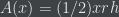

The Equation of a Catenary
In the above section, essentially the same method was used again and again to solve different problems. As an example of a different way to apply SIA in single-variable calculus, in this section I’ll outline how the equation of a catenary may be derived in it. The full derivation is in [Bell2].)
To do this, we’ll need the existence of functions 


Axiom (Scheme) 6. For every 


(We can actually go further. For every 


Suppose that we have a flexible rope of constant weight 


Let 

Let 

Let
Let 


1. A force of magnitude 

2. A force of magnitude 

3. A force of magnitude 

By resolving these forces horizontally and using microcancellation, one can show that the horizontal component of the tension (that is, 

By resolving these forces vertically and using microcancellation and the fact that 

Finally, by combining the results of the previous two paragraphs and using the fact that 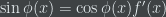

Solving differential equations symbolically is the same in SIA as it is classically, since no infinitesimals or limits are involved. In this case, the answer turns out to be

if we add the initial condition 

I’ll include a post on multivariable calculus later.

I don’t understand a word/character/symbol but it looks great!
I recently became very interested in smooth infinitesimal analysis, and found your article a useful guide when trying to understand some of the earlier works (Kock, Reyes-Moerdijk, etc.).
However, there is something that bothers me about this setup, and I wonder if you have any ideas on it. Specifically, the problem is Axiom 5. This axiomatizes the fundamental theorem of calculus! Is there no way to define an area function using infinitesimals, then show that its derivative is the original function?
I think the idea of taking as an axiom “every curve is made up of infinitesimally small line segments” a beautiful concept, but it seems to me to be giving up too much to also have to axiomatize the existence of an anti-derivative.
Do you know of any way to not have to take this as an axiom?
Hi Geoff,
I’m glad you liked the article and find the subject interesting!
Axiom 5 doesn’t really axiomatize the fundamental theorem of calculus, since all Axiom 5 says is that antiderivatives of functions exist. The fundamental theorem of calculus says something more: it says that not only do antiderivatives of (suitable) functions exist, but that furthermore the function
  giving the (signed) area under the graph of
  from
from  to
to  is a specific example of an antiderivative. (Also, that all other antiderivatives are equal to
  plus some constant.)
The notation is confusing though, because in Axiom 5, I said that antiderivatives of functions exist, and furthermore I denoted the antiderivative of which takes the value
  on input
  by
by  . This could be confusing, because normally
  is defined as a Riemann sum, which is the classical formalization of the “area” concept, and so with that notation, the statement that the derivative of
  is
is  is indeed the fundamental theorem of calculus. But with the notation I used in this article, it’s just a definition.
As an aside, you can prove a version of the fundamental theorem of calculus in smooth infinitesimal analysis, in much the same way that you can find the area of a cone.
If you want to not take the existence of antiderivatives as an axiom, you might want to take a look at Bell’s book “A Primer on Smooth Infinitesimal Analysis,” which does a lot of stuff without that axiom, but in its place he assumes that if and
and  then
then  .
.
Ah, of course you’re right. I think I was confused by the notation. Thanks for the quick reply.
I guess my next question would be: how does one define the “area under a curve” function? I assume we would like to do it without limits.
Now that I look over the above again, I notice that there’s something similar with the arc length function: you mention that it’s not formally defined, so instead work with what reasonable properties it should have. But there has to be some nice way to formally define these notions; perhaps I just need to get Bell’s book.
As a side note, I’m amazed by how much more elegant some of the proofs with smooth infinitesimal analysis are than with regular calculus. In particular, the proofs of the product and chain rules are so much nicer than their usual counterparts.
I definitely agree that the proofs in smooth infinitesimal analysis are much nicer than in classical calculus; that’s the main reason why I like it.
You define the “area under a curve” function in a similar way to arclength as follows: You show that, given , there is a unique function
  (to be interpreted as the area under the curve
  from
from  to
to  such that: for all
  ,
,  and, if
  is linear on
  , then
  is the appropriate value (i.e., the formula for the area of a trapezoid:
  . You can then prove that there is a unique function
  with these properties, and it’s
  .
.
The way area is dealt with in smooth infinitesimal analysis (i.e., isolate some conditions that an area function must have, then prove there is a unique function satisfying those conditions) is not so different from what is done in the classical case. The problem is that it’s done over again for each problem type: that is, you use it once to determine the area of a cone, then once again to prove the fundamental theorem of calculus, etc.
If I understand your question right, you’re wondering if you can do it once and for all. That is, can you prove that there is a unique function assigning to subsets of, say, an element of
  satisfying the appropriate conditions. I don’t know, but I would guess that the answer is “no.” I would have to think some more about that (and probably learn some more first!). If you have any thoughts, let me know.
Can these notions be extended to the calculus of variations?
Robert, I wouldn’t call myself an expert, but yes: the fact that smooth infinitesimal analysis is modeled in a topos means “smooth spaces” include function spaces, where the calculus of variations naturally lives. For instance, one has a smooth space of smooth paths between two points of a manifold, and it is an easy proposition that tangent vectors in that smooth space are equivalent to vector fields along a chosen path. One can go on to perform analysis on smooth functionals on such function spaces within this setting in a very intuitive fashion.
Have you seen Keisler text book
Elementary Calculus: An Infinitesimal Approach
1976, 1986 available on line free at
http://www.math.wisc.edu/~keisler/calc.html